Pharmacokinetic Modeling

Getting There

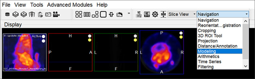
The Modeling operator can be accessed via the tool pull-down menu on VivoQuant’s front panel.

Function

For more on the function of the Modeling operator, see the Modeling operator page.

Input/Reference Function

Every tissue model requires the input of an additional temporal curve, either as an arterial input function or concentration of a reference tissue. These temporal data may be derived from image data directly or from acquired samples. The operator supports input and computation of parent fraction samples, plasma fraction samples, whole blood concentration, and plasma concentration. In addition, these data can be stored and retrieved from disk and from an iPACS.

Parent/Plasma Fraction

The experimentalist may have acquired blood samples throughout the subject’s scanning session. From these samples, the ratio of unmetabolized tracer to the sum of unmetabolized tracer and its derivative metabolites can be measured and used to account for the dynamic nature of available tracer. This is also known as the parent fraction or plasma free fraction. Without it, the tissue model must assume that metabolism of the tracer is negligible. Whether measured, simulated, or estimated, the parent fraction can play an important role in accurate estimation of tissue kinetics downstream. Similarly, the fraction of plasma to whole blood (including red blood cells) has been shown to be an important factor in the estimation of an appropriate arterial input function [1]. The fraction modeling can be selected from the dropdown of models or from the Operator menu.

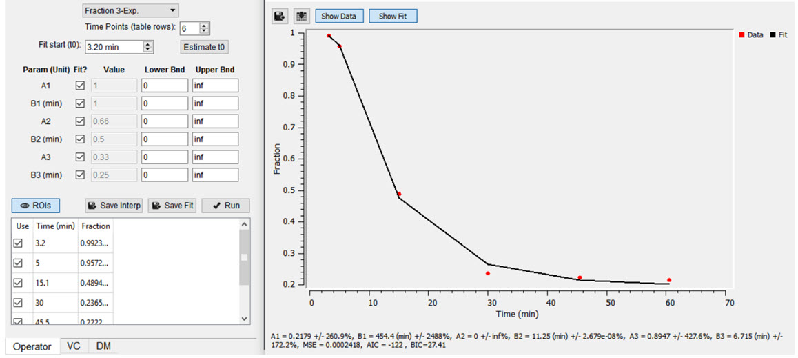
Both plasma and parent fraction data can be input using the same tool. Towards the bottom of the operator, space is provided for a table of fraction data. There are 3 columns. The first one can be used to exclude specific time points from the table. The second column contains the time of each sample in units of minutes. The last column contains free fraction values, assumed to have a value between zero and one. Users can choose to use a linear interpolation of the points or fit a sum of exponentials to the provided points. The Save Interp button can be used to save the points as is, at which point the tool will prompt the user for a name to give the saved curve. If this option is chosen, the operator will prepend a value to time=zero, assuming that the fraction is equal to one at that time. After the last provided time point, the value is assumed to remain constant equal to the last fraction value.

Users may want to smooth the fraction points with a sum of exponentials. Up to 3 exponentials can be used to fit the curve. If less exponentials are desired, users can fix model parameters for one or more of the exponentials (i.e. fix A3=0 and B3=0) [2]. To do so, use the Run button to estimate model parameters under the input conditions provided by the user.

Once you are satisfied with the model estimates, click on Save Fit while the estimate plots are open to save the current model-estimated fraction curve to the list.

Model Assumptions

This model makes the following assumptions:

• The exponential decay begins at user-provided t0
• Provided fraction measurements lie between zero and one

References

[1] “Red blood cells: a neglected compartment in pharmacokinetics and pharmacodynamics”. Hinderling. Pharmacol Rev, 1997. Link.

[2] “Optimal Metabolite Curve Fitting for Kinetic Modeling of 11C-WAY-100635”. Wu, et al. JNM, 2007. Link.

Arterial Input Function

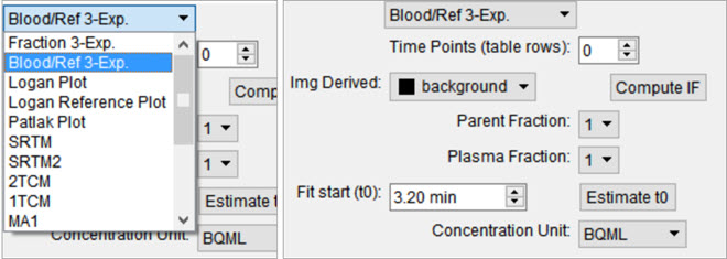
An Arterial Input Function (AIF) is required for Logan, Patlak, 1- and 2-tissue compartment, and MA1 analysis. To add time points to an AIF, begin by selecting Blood/Ref 3-Exp from the list of models.

Similar to the parent fraction, users can select to save a linear interpolation of points or a smooth model estimate of AIF samples. Either way, samples should be input into the table of values as a first step. This may be done with a copy/paste from an external spreadsheet program or by incrementing the Time Points (table rows) number and manually editing the table. The table assumes a structure with the number of rows equal to the number of samples. Each sample has three columns. The first column indicates whether that sample should be excluded or not. The second column contains the time (in minutes) at which sample was measured. Times should be consistently relative to the same reference start time as the final modeled time activity curves. The third column contains the measured concentration value at that time. If parent or plasma fraction data are available and applicable to the provided samples, select them from the dropdown. If none is selected, the fraction is assumed to be one for the entirety of the time activity curve. If image derived samples are desired, the user may also compute the samples directly from the average concentration values with ROIs in the loaded image. To do this, select the appropriate region from the dropdown and click on the *Compute IF button. For more information on segmenting regions of interest from an image, see the 3D ROI tool.

If a sum of exponentials model for the samples is desired for smoothing the data, click on Run to estimate exponential parameters for the data. Before doing so, it may be important to select an appropriate t₀ value. This is best estimated from the samples themselves with the Estimate t₀, which will set t₀ to the time point where the maximum concentration occurs in the samples. The linearly interpolated samples or model fit may be saved for use in tissue modeling with the Save Interp or Save Fit buttons, respectively.

Reference Tissue Compartment

The reference tissue compartment concentrations can be readily computed similar to the Arterial Input Function (AIF). Like the AIF, you may input the concentrations from a spreadsheet or by manual input; however, it is more likely you will want to derive the concentration values from a reference region segmented on the loaded images. For more information on segmentation techniques in VivoQuant, see the 3D ROI Tool page. Begin by navigating to the Blood/Ref 3-Exp. model in the operator. Next, select the appropriate region of interest in the Img Derived dropdown.

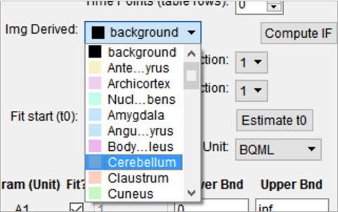
The Compute IF button will compute the average concentration in the selected region and populate the table, one row for each volume loaded. The time points are computed from the image acquisition times and frame durations, set to the midpoint of each frame, and relative to the start of the dynamic scan. Should the temporal information be missing from the image data, this can be added using the Frame Time Editor, found in the Tools menu. A sum of exponentials model can also be estimated from the table data. Ensure that the parent/plasma fraction inputs are disabled by setting their respective dropdown setting to 1. To save a linear interpolation of the concentrations, click on the Save Interp button. Should you want to fit a sum of exponentials, begin by specifying an appropriate t₀ parameter, which can typically be estimated using the Estimate t₀ button. Fitting the sum of exponentials model can be done with the Run button, at which point you will be able to save the fit using the Save Fit button.

Saving and Loading of Fraction, AIF, and Reference Region Data

All temporal curves can be saved with the Save Interp or Save Fit buttons. When they are saved, their user-provided name appears in the dropdown of Saved Curves.

Controls next to the dropdown are available for saving, loading, and viewing the curves. The menu provides options for storing the temporal data to/from the iPACS or as a spreadsheet on your local hard drive. This is particularly useful to avoid re-entry of the information should you want to re-run analysis at a later date. The menu is an additional tool for the user to store the current linearly interpolated samples or modeled data into the list of saved curves. The button clears the currently selected temporal curve from the list. Lastly, the button opens a new dialog window showing a plot of the temporal curve which can be saved as a local image for quality control.

Additional Resources

• “Emission Tomography: The Fundamentals of PET and SPECT”, Miles Wernick & John Aarsvold. Elsevier, 2004. Print.
• “Fractions of unchanged tracer in plasma”, Vesa Oikonen. Turku PET Center website. Link
• “Converting blood TAC to plasma TAC”, Vesa Oikonen. Turku PET Center website. Link
• “Blood sampling in PET studies”, Vesa Oikonen. Turku PET Center website. Link
• “Arterial input function from PET image”, Vesa Oikonen. Turku PET Center website. Link

Models

Two-Tissue Compartment Model (2TCM)

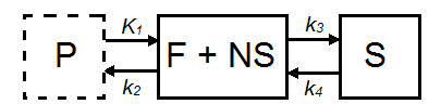
The 2TCM is a three-compartment model that includes two tissue compartments: one tissue compartment represents free and nonspecifically bound tracer within the tissue (referred to as nondisplaceable), and the other tissue compartment represents specifically bound tracer within the tissue. The third compartment represents tracer within the arterial plasma.

Parameter	Description
CND(t)	Concentration in F + NS compartment, nodisplaceable tracer.
CS(t)	Concentration in specifically bound (S) compartment.
Cp(t)	Concentration in plasma (P) compartment.
K1(mL*cm3*min-1)	Transfer of ligand from arterial plasma to tissue.
k2 (min-1)	Transfer of ligand from tissue to arterial plasma.
k3(min-1)	Transfer of ligand into specifically bound compartment.
k4 (min-1)	Transfer of ligand out of specifically bound compartment.

For those tracers for which a compartmental model is appropriate, estimation of the rate constants provides valuable information about tracer uptake and binding [1]. Due to the difficulty of reliably estimating all four parameters of the 2TCM, lumped or macroparameters are often employed. Macroparameters are rate constants which are functions of individual microparameters (e.g. K₁, k₂, k₃ and k₄). One such macroparameter that is estimated by the 2TCM is the total volume of distribution, V_T.

When the 2TCM is applied to image data with a reference region, the distribution volume ratio (DVR) can be calculated: DVR = V_T/V_ND, where V_ND is the estimated distribution volume in a region that is devoid of the target site or receptor (often called the reference region or nondisplaceable region). Binding potential (BP_ND) can then be calculated by BP_ND = DVR - 1.

Model Assumptions

This model makes the following assumptions:

• The tracer binds reversibly.
• Nonspecifically bound ligand equilibrates rapidly with free tissue ligand.
• Compartmental model assumptions:
  • The tracer kinetics or behavior can be represented by a compartmental model.
  • Tracer concentration within each compartment is well-mixed and does not vary spatially.
  • First-order kinetics can describe exchange of ligand between compartments.

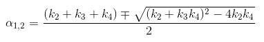
The 2TCM is currently implemented in VivoQuant using a basis function method approach [2] and unweighted fitting in this basis function method,

Required Inputs

This model requires the following inputs:

• Metabolite-corrected arterial plasma input curve.
• ROI(s) or voxels.

Outputs

Region-level analysis:

• Plot of data from each ROI with 2TCM fit.
• V_T, K₁, k₂, k₃, k₄, mean-squared error (MSE) of fit, Θ₁, and Θ₂ are shown when the cursor is hovered over the model fit plot.
• V_T, K₁, k₂, k₃, k₄, mean-squared error (MSE), data and 2TCM fit for each ROI can be saved out to .csv

References

[1] “A quantitative model for the in vivo assessment of drug binding sites with positron emission tomography”. Mintun, et al. Ann Neurol, 1984. Link.

[2] “Kinetic modelling using basis functions derived from two-tissue compartmental models with a plasma input function: general principle and application to [18F]fluorodeoxyglucose positron emission tomography”. Hong, et al. NeuroImage, 2010. Link.

Additional Resources

“Compartmental Models”, Vesa Oikonen. Turku PET Center website. Link.

One-Tissue Compartment Model (1TCM)

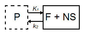
The 1TCM is a two-compartment model that includes one compartment representing tracer within the tissue (free and nonspecifically bound tracer which together are referred to as nondisplaceable tracer) and one compartment representing tracer within the arterial plasma [1].

Parameter	Description
CND(t)	Concentration in F + NS compartment, nondisplaceable tracer.
Cp(t)	Concentration in plasma (P) compartment.
K1 (mL*cm3*min-1)	Transfer of ligand from arterial plasma to tissue.
k2 (min-1)	Transfer of ligand from tissue to arterial plasma.
VT = K1/k2	Total volume of distribution.

For tracers for which a compartmental model is appropriate, estimation of the rate constants provides valuable information about tracer uptake [2]. The 1TCM is generally easier and less computationally intensive to solve than the 2TCM, because it is a simpler model and has fewer parameters. Additionally, the 1TCM model parameters can generally be estimated with better identifiability than the 2TCM model parameters.

In some cases, the exchange of tracer between the nondisplaceable and bound tissue is sufficiently fast, so the two cannot be distinguished kinetically. In these cases, the nondisplaceable and bound tissue compartments may be collapsed into one compartment that represents both the nondisplaceable and specifically bound tracer within the tissue [3]. In these cases, apparent transfer of ligand from tissue to arterial plasma is represented by the parameter k_2a and V_T = K₁/k_2a.

When a tracer that specifically binds to a target can be represented by a 1TCM as above, and has a reference region the distribution volume ratio (DVR) can be calculated: DVR = V_T/V_ND, where V_ND is the estimated distribution volume in the reference region. Binding potential (BP_ND) can then be calculated by BP_ND = DVR - 1.

Model Assumptions

This model makes the following assumptions:

• The tracer binds reversibly.
• Nonspecifically bound ligand equilibrates rapidly with free tissue ligand.
• Compartmental model assumptions:
  • The tracer kinetics or behavior can be represented by a compartmental model.
  • Tracer concentration within each compartment is well-mixed and does not vary spatially.
  • First-order kinetics may be used to describe exchange of ligand between compartments

Required Inputs

This model requires the following inputs:

• Metabolite-corrected arterial plasma input curve
• ROI(s) or voxels

Outputs

Region-level analysis:

• Plot of data from each ROI with 1TCM fit.
• V_T, K₁, k₂, and mean-squared error (MSE) of fit are shown when the cursor is hovered over the model fit plot.
• V_T, K₁, k₂, and mean-squared error (MSE) of fit, data, and 1TCM fit for each ROI can be saved out to .csv.

Voxel-level analysis

• Plot of data for each voxel with 1TCM fit. Select the voxel for which you would like to see the model fit by clicking on it with the image viewer.
• V_T, K₁, k₂, and mean-squared error (MSE) of fit are shown when the cursor is hovered over the model fit plot.
• Parameter maps for V_T, K₁, k₂, and mean-squared error (MSE).

References

[1] “Kinetic modeling in positron emission tomography”. Morris, et al. In: Emission Tomography: The Fundamentals of PET and SPECT (Eds: wermick MN, Aarsvold JN). 2004.

[2] “Comparison of methods for analysis of clinical [11C]raclopride studies”. Lammerstsma, et al. JCBFM, 1996. Link

[3] “Kinetic modelling using basis functions derived from two-tissue compartmental models with a plasma input function: general principle and application to [18F]fluorodeoxyglucose positron emission tomography”. Hong, et al. NeuroImage, 2010. Link.

Additional Resources

“Compartmental Models”, Vesa Oikonen. Turku PET Center website. Link

Logan Graphical Method (Logan Plot)

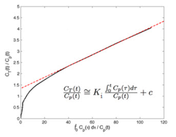
The Logan Graphical Method [1] was developed for reversibly bound tracers based on the Patlak method for irreversibly bound tracers [2]. The Logan method proposes that after some time t*, the plot of

vs.

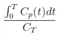
where C_T is the concentration of the tracer in the tissue and C_P is the concentration of the tracer in the metabolite-corrected arterial plasma, becomes linear with slope equal to the total volume of distribution, V_T.

When the Logan Plot is applied to image data with a reference region, the distribution volume ratio (DVR) can be calculated: DVR = V_T/V_ND, where V_ND is the estimated distribution volume in the reference region. BP_ND is related to DVR by BP_ND = DVR - 1

The Logan Plot is a rearrangement of tracer kinetic equations to yield a useful linear equation. However, the mapping of transformed variables is nonlinear in C_T(t), and this results in an underestimation of V_T which becomes more pronounced with larger true V_T and increased noise [1,3]. Therefore, the Logan graphical method may not be the best method to use when data are noisy, and other methods should be considered.

Model Assumptions

This model makes the following assumptions:

• The tracer binds reversibly
• After some time t* the slope of the plot of vs. approaches linearity.

Required Inputs

This model requires the following inputs:

• Metabolite-corrected arterial plasma input curve
• ROI(s) or voxels
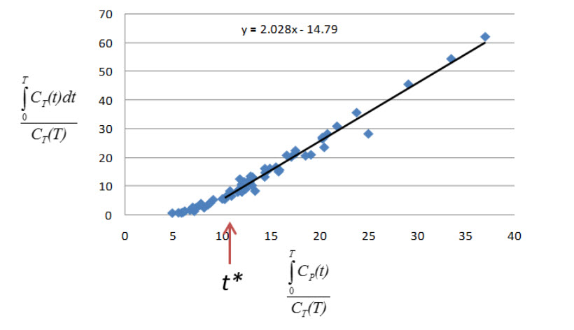
• t* (in scan time)
  • Selection of t*: The Logan plot as implemented in VivoQuant requires that the user inputs the t*, which defines the time at which the plotted data become linear. In VivoQuant the default t* value is 0. This is likely not the appropriate value for your experiment. t* values are tracer dependent. For characterized tracers, we suggest reviewing the literature to see which t* values have been used in Logan method. The simplest way to select a reasonable t* value for your data is to run the model once with the default t* value, review the Logan plots to find the point at which they become linear (t*), then re-run the model with the appropriate t* (in scan time) value.

Outputs

Region-level analysis

• Logan plot with line fit for each voxel. Select the voxel for which you would like to see the Logan plot by clicking on it within the image viewer.
• V_T, fitted line intercept, and mean-squared error (MSE) of fit are shown when the cursor is hovered over the Logan plot.
• Parameter maps for VT, fitted line intercept, and MSE.

References

[1] “Kinetic modeling in positron emission tomography”. Morris, et al. In: Emission Tomography: The Fundamentals of PET and SPECT (Eds: wermick MN, Aarsvold JN). 2004.

[2] “Comparison of methods for analysis of clinical [11C]raclopride studies”. Lammerstsma, et al. JCBFM, 1996. Link

[3] “Effects of Statistical Noise on Graphic Analysis of PET Neuroreceptor Studies”. Slifstein and Laruelle. JNM, 2000. Link

Additional Resources

“Multiple Time Graphical Analysis (MTGA)”, Vesa Oikonen. Turku PET Center website. Link

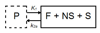
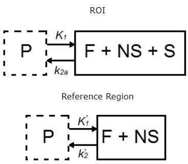
Simplified Reference Tissue Model (SRTM)

The simplified reference tissue model (SRTM) [1] allows for quantification of tracer kinetics without requiring an arterial input function. SRTM is a numerically robust model which assumes that the tracer can be represented by 1-tissue compartment models in both the ROIs and the reference region.

Parameter	Description
CT(t)	Concentration in F + NS + S compartment.
CND(t)	Concentration in F + NS compartment, nondisplaceable tracer.
CP(t)	Concentration in plasma (P) compartment.
K1 (mL*cm3*min-1)	Transfer of ligand from arterial plasma to tissue.
k2a (min-1)	Apparent transfer of ligand from tissue to arterial plasma.
K1’ (mL*cm3*min-1)	Transfer of ligand from arterial plasma to reference tissue.
k2’ (min-1)	Transfer of ligand from reference tissue to arterial plasma.

Model Assumptions

This model makes the following assumptions:

• The tracer binds reversibly.
• Tracer concentration in all regions or voxels-of-interest as well as the reference region (see below) can be represented by a 1-tissue compartment model.
• A region/tissue exists which is devoid of the target site/receptor. We call this region the reference region. It represents the concentration of the tracer which is free in tissue and/or bound to off-target sites (non-specific binding). An ideal reference region is a) devoid of the target site/receptor, and b) has the same concentration of tracer free in tissue and nonspecifically bound as the ROI.

Required Inputs

This model requires the following inputs:

• Reference tissue curve.
• ROI(s) or voxels.

Outputs

Region-level analysis

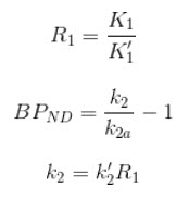
• Plot of data from each ROI with SRTM fit.
• BP_ND, R₁,k₂,k₂’, and mean-squared error (MSE) of fit are shown when the cursor is hovered over the model fit plot.
• BP_ND, R₁,k₂,k₂’, and mean-squared error (MSE), data and SRTM fit for each ROI can be saved out to .csv.

Voxel-level analysis

• Plot of data for each voxel with SRTM fit. Select the voxel for which you’d like to see the model fit by clicking on it with the image viewer.
• BP_ND, R₁,k₂,k₂’, and mean-squared error (MSE) of fit are shown when the cursor is hovered over the model fit plot.
• Parameter maps for BP_ND, R₁,k₂,k₂’ and MSE.

References

[1] “Simplified reference tissue model for PET receptor studies”, Lammerstma and Hume. NeuroImage, 1996. Link

[2] “The simplified reference tissue model: model assumption violations and their impact on binding potential”, Salinas, et al. JCBFM, 2015. Link

[3] “Parametric imaging of ligand-receptor binding in PET using a simplified reference region model”. Gunn, et al. NeuroImage, 1997. Link

Additional Resources

“Reference region input compartmental models”, Vesa Oikonen. Turku PET Center website. Link.

Simplified Reference Tissue Model 2 (SRTM2)

SRTM2 is a two-pass version of SRTM that attempts to reduce noise in parametric images by fitting all voxels with a fixed, global k₂’ [1]. In practice, SRTM estimates k₂’ for every voxel or region, but since there is only one reference region, in principle there is only one true k₂’ value [1]. Fixing k₂’ reduces the number of parameters estimated and thus reduces noise in parametric images [1]. However, this improvement in precision may come at the price of an increase in bias [1].

Model Assumptions

This model makes the following assumptions:

• The tracer binds reversibly
• Tracer concentration in all regions or voxels-of-interest as well as the reference region (see below) can be represented by a 1-tissue compartment model.
• A region/tissue exists which is devoid of the target site/receptor. We call this region the reference region. It represents the concentration of the tracer which is free in tissue and/or bound to off-target sites (non-specific binding). An ideal reference region is a) devoid of the target site/receptor, and b) has the same concentration of tracer free in tissue and nonspecifically bound as the ROI.
• There is only one true k₂’ value. k₂’ is the rate of tracer efflux from the reference region to the plasma.

Required Inputs

This model requires the following inputs:

• Reference tissue curve.
• ROI(s) or voxels.
• A fixed k₂’
• Selection of a fixed k₂‘: The value to which to fix k₂’ should be selected based on the tracer and the experiment. For characterized tracers, we suggest reviewing the literature to see how the fixed k₂’ has been selected in different studies and the effect of the method to fix k₂’ on SRTM2 parameter estimates. Generally, k₂’ can be fixed to the median value estimated by a first-pass of SRTM from all voxels with a BPND value > a set minimum [3,4] or all voxels with a BPND value within a given range [5]. The idea behind using BPND values to select voxels for inclusion in the median is to exclude voxels which maybe represent noise or have poor SRTM fit. For most tracers there is a range of physiologically-relevant BPND values. Values outside of that range may be non-physiological. Other studies have fixed k₂’ to the population average value estimated from a 1-tissue compartment model fit to the reference region [3] or estimated k₂’ for each subject by a simultaneous SRTM fit including all target regions with coupled k₂’ [3,6]. SRTM fit with coupled k₂’ is not currently available in VivoQuant.

Outputs

Region-level analysis

• Plot of data from each ROI with SRTM2 fit.
• BP_ND, R₁,k₂a, and mean-squared error (MSE) of fit are shown when the cursor is hovered over the model fit plot.
• BP_ND, R₁,k_2a, and mean-squared error (MSE), data and SRTM2 fit for each ROI can be saved out to .csv.

Voxel-level analysis

• Plot of data for each voxel with SRTM2 fit. Select the voxel for which you’d like to see the model fit by clicking on it with the image viewer.
• BP_ND, R₁, k_2a, and mean-squared error (MSE) of fit are shown when the cursor is hovered over the model fit plot.
• Parameter maps for BP_ND, R₁, k_2a, and MSE.

References

[1] “Noise reduction in the simplified reference tissue model for neuroreceptor functional imaging.”, Wu and Carson. JCBFM, 2002. Link

[2] “Parametric imaging of ligand-receptor binding in PET using a simplified reference region model”. Gunn, et al. NeuroImage, 1997. Link

[3] “Tracer kinetic modeling of [(11)C]AFM, a new PET imaging agent for the serotonin transporter”. Naganawa, et al. JCBFM, 2013. Link

[4] “Parametric Imaging and Test-Retest Variability of 11C-(+)-PHNO Binding to D2/D3 Dopamine Receptors in Humans on the High-Resolution Research Tomograph PET Scanner”, Gallezot, et al. JNM, 2014. Link

[5] “Kinetic modeling of the serotonin 5-HT1B receptor radioligand [11C]P943 in humans”. Gallezot, et al. JCBFM, 2010 Link

[6] “Assessment of striatal dopamine D2/D3 receptor availability with PET and 18F-desmethoxyfallypride: comparison of imaging protocols suited for clinical routine”. Amtage, et al. JNM, 2012. ¨Link

Additional Resources

“Reference region input compartmental models”, Vesa Oikonen. Turku PET Center website. Link.

Logan Non-Invasive Graphical Method (Logan reference plot)

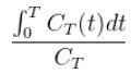
The Logan non-invasive graphical method [1] was developed for reversibly bound tracers based on the Logan graphical method and Patlak method for irreversibly bound tracers [2,3]. The Logan reference method proposes that after some time t*, the plot of

vs.

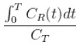
(where C_T is the concentration of the tracer in the tissue and C_R is the concentration of the tracer in the reference region) becomes linear with slope equal to the distribution volume ratio (DVR). Binding potential (BP_ND) is related to DVR by BP_ND = DVR - 1.

The Logan plot is a rearrangement of tracer kinetic equations to yield a useful linear equation. However, the mapping of transformed variables is nonlinear in C_T(t), and this results in an underestimation of DVR which becomes more pronounced with larger true DVR and increased noise [1,4]. Therefore, the Logan graphical method may not be the best method to use when data are noisy, and other methods should be considered.

Method Assumptions

This model makes the following assumptions:

• The tracer binds reversibly.
• A region/tissue exists which is devoid of the target site/receptor. We call this region the reference region. It represents the concentration of the tracer which is free in tissue and/or bound to off-target sites (non-specific binding). An ideal reference region is a) devoid of the target site/receptor, and b) has the same concentration of tracer free in tissue and nonspecifically bound as the ROI.
• After some time t* the slope of the plot of vs. approaches linearity.

Required Inputs

This model requires the following inputs:

• Reference tissue curve.
• ROI(s) or voxels.
• t* (in scan time)
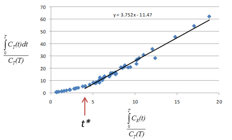
  • Selection of t*: The Logan reference plot as implemented in VivoQuant requires that the user inputs the t* which defines the time at which the plotted data become linear. In VivoQuant, the default t* value is 0. This is likely not be the appropriate value for your experiment. t* values are tracer dependent. For characterized tracers, we suggest reviewing the literature to see which t* values have been used in Logan reference method. The simplest way to select a reasonable t* value for your data is to run the model once with the default t* value, review the Logan reference plots to find the point at which they become linear (t/), then re-run the model with the appropriate *t/* (in scan time) value.

Outputs

Region-level analysis

• Logan plot with line fit for each ROI.
• DVR, fitted line intercept, and mean-squared error (MSE) of fit are shown when the cursor is hovered over the Logan plot.
• DVR, fitted line intercept, and transformed Logan space data for each ROI can be saved out to .csv.

Voxel-level analysis

• Logan plot with line fit for each voxel. Select the voxel for which you would like to see the Logan plot by clicking on it within the image viewer.
• DVR, fitted line intercept, and MSE of fit are shown when the cursor is hovered over the Logan plot.
• Parameter maps for DVR, fitted line intercept, and MSE.

References

[1] “Distribution volume ratios without blood sampling from graphical analysis of PET data”. Logan, et al. JCBFM, 1996. Link

[2] “Graphical analysis of reversible radioligand binding from time-activity measurements applied to [N-11C-methyl]-(-)-cocaine PET studies in human subjects”. Logan, et al. JCBFM, 1990. Link

[3] “Graphical evaluation of blood-to-brain transfer constants from multiple-time uptake data”. Patlak, et al. JCBFM, 1983. Link

[4] “Effects of Statistical Noise on Graphic Analysis of PET Neuroreceptor Studies”. Slifstein and Laruelle. JNM, 2000. Link

Additional Resources

“Multiple Time Graphical Analysis (MTGA)”, Vesa Oikonen. Turku PET Center website. Link

Patlak Analysis (Patlak Plot)

Patlak analysis is rearrangement of tracer kinetic equations to yield a useful linear equation [1]. Patlak analysis proposes that after some time t*, the plot of

vs.

where C_T is the concentration of the tracer in the tissue and C_P is the concentration of the tracer in the metabolite-corrected arterial plasma, becomes linear with slope equal to the net influx rate constant, K_i. The rate constant K_i represents influx and trapping of the tracer into the tissue [1,2].

In terms of a two-tissue compartment model where k₄ = 0 because the tracer is irreversibly trapped, K_i =

Model Assumptions

This model makes the following assumptions:

• The tracer binds irreversibly
• After some time t*, the slope of the plot of vs. approaches linearity.

Required Inputs

This model requires the following inputs:

• Metabolite-corrected arterial plasma input curve.
• ROI(s) or voxels
• t* (in scan time)
  • Selection of t*: The Patlak plot as implemented in VivoQuant requires that the user inputs the t* which defines the time at which the plotted data become linear. In VivoQuant the default t* value is 0. This is likely not be the appropriate value for your experiment. t* values are tracer dependent. For characterized tracers, we suggest reviewing the literature to see which t* values have been used in Patlak analysis. The simplest way to select a reasonable t* value for your data is to run the model once with the default t* value, review the Patlak plots to find the point at which they become linear (t*), then re-run the model with the appropriate t* (in scan time) value.

Outputs

Region-level analysis

• Patlak plot with line fit for each ROI.
• K_i, fitted line intercept (V), and mean-squared error (MSE) of fit are shown when the cursor is hovered over the Patlak plot.
• K_i and transformed Patlak space data for each ROI can be saved out to .csv.

Voxel-level analysis

• Patlak plot with line fit for each voxel. Select the voxel for which you would like to see the Patlak plot by clicking on it within the image viewer.
• K_i, fitted line intercept (V), and mean-squared error (MSE) of fit are shown when the cursor is hovered over the Patlak plot.
• Parameter maps for K_i, fitted line intercept (V), and MSE.

References

[1] “Graphical evaluation of blood-to-brain transfer constants from multiple-time uptake data”. Patlak, et al. JCBFM, 1983. Link.

[2] “Net Influx Rate, (Ki)”, Vesa Oikonen. Turku PET Center website. Link.

Additional Resources

“Multiple Time Graphical Analysis (MTGA)”, Vesa Oikonen. Turku PET Center website. Link.