The MIP (Maximum Intensity Projection) control can be used to manipulate the active 3D rendered volume. See MIP Explained for a more detailed description of how the MIP is generated. This tool also allows the user to automatically rotate the 3D volume and create custom movements that can be exported as videos or gifs.
Getting There
There are three different methods for reaching the MIP Control window. The first method is to use the MIP Control thumbnail in the Main Window.
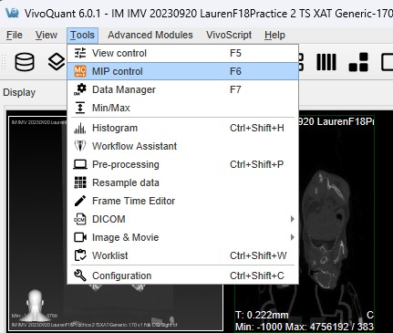
The second method is to go to MIP Control under the Tools menu.
The third method is to use the keyboard shortcut F6. For a complete list of keyboard shortcuts, see Keyboard Shortcuts.
Function
The MIP Control window provides a variety of options for manipulating the MIP and the appearance of open data sets in VivoQuant’s main window.
Main Controls
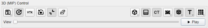
| Icon | Function | Description |
|---|---|---|
| Save / Load Settings | Provides an option to save the current settings or load previously saved 3D settings. | |
| Auto Update | Provides an option to enable or disable automatic settings update. | |
| Force Refresh | Forces re-rendering of the 3D view. | |
| Reset Camera | Resets the camera of the 3D view to its initial position. | |
| Expand vs Contract View | Expands the 3D view bounds to aid in rotation. | |
| Perspective vs Orthogonal Projection | Switching projection mode; useful for treating the 3D view more as a slice viewer when looking down an axis. | |
| Bounding Box | Enables 3D bounding box and clipping. | |
| Gradient Box | If enabled, replaces black background with gradient grey background. | |
| Toggle MIP | Toggles the classic MIP in the 3D view. | |
| Toggle MPR | Toggles Multi-planar reconstruction (MPR) view in 3D view. Hold down to toggle background transparency. | |
| Orientation Cube | Toggles orientation cube in the 3D view. Hold down to select the orientation model: Default, Human, Human Head, Rodent or Rodent Head. | |
| Annotation | Toggles visible annotations in the 3D view. | |
| Quality | Changes performance of 3D view by optionally down-sampling the image. Hold this button down to specify the resolution: Fine, Standard, or Fast. |
See 3D View Shortcuts for keyboard shortcuts related to 3D rendering.
Camera Controls
See 3D View Shortcuts for keyboard shortcuts related to camera controls.
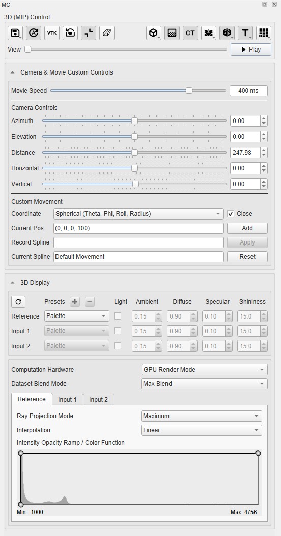
Camera & Movie Custom Controls
The application provides several UI elements to control camera playback for 3D rendering. By default, when the user presses the Play button, the camera rotates around the Z-axis in fixed increments of 3 degrees per step. In addition to the default rotation mode, the user can define a custom camera trajectory using spline control points. Each control point records the full camera pose, including position and orientation. These control points define the path the camera follows during playback. The camera pose for each control point can be set in two ways:
- Mouse interaction – Manually adjust the camera to find an optimal viewpoint.
- Fine-grained numeric controls – Sliders and spin boxes allow precise manipulation of the camera pose.
The movie playback speed is also configurable. When exporting a 3D rendered movie, the current camera playback configuration (trajectory, pose parameters, and speed) is used.
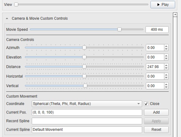
Camera Pose Controls
The camera pose is controlled using the following parameters, each exposed as a slider + spin box pair:
| Azimuth | Controls the horizontal rotation of the camera around the target (rotation about the vertical axis at the focal point). |
| Elevation | Controls the vertical rotation of the camera (rotation about the horixontal axis at the focal point). |
| Distance | Controls the camera’s distance from the focal point (zoom in/out in world space). |
| Horizontal Offset | Translates the camera target horizontally (left/right) in the scene. |
| Vertical Offset | Translates the camera target vertically (up/down) in the scene. |
Sliders provide coarse adjustments, while spin boxes allow precise numeric entry.
Custom Movement (Spline Recording)
The Custom Movement section allows recording and applying camera trajectories:
| Current Position | Shows the current camera position. |
| Add Button | Records the current camera pose as a control point in the recorded spline. |
| Recorded Spline List | Displays the serialized list of recorded control points. |
| Apply Button | Loads the recorded spline into the active spline field, making it the current playback trajectory. |
Once applied, this spline is used for camera playback and for exporting rendered movies.
3D Display
The 3D display allows for fine tuning of some of the parameters offered by our renderers. Although the main use case is typically a MIP (Maximum Intensity Projection), the 3D display supports other rendering techniques that can prove useful in certain scenarios. Some of which include gradient detection and surface rendering.
Some functions include:
- Opacity and color transfer editing function by means of image histograms.
- CPU and GPU based volume rendering pipelines.
- Interpolation mode selector to change the quality of the 3D rendering.
- Ability to save settings to disk and load previously saved 3D settings.
Transfer Function
Transfer functions are tools for assigning optical properties to scalar volume data sets. For direct volume rendering, for example, opacity can be set depending on the gray value at a given voxel position.
VivoQuant’s 3D Viewer allows for editing opacity and color transfer functions by using image histograms and other volume rendering options.
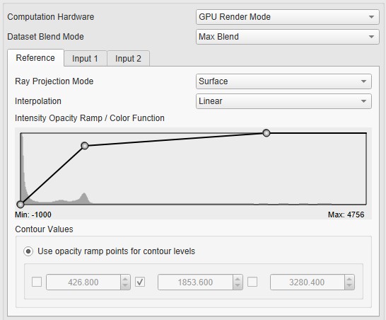
-
Computation hardware: This option allows users to choose the desired processing platform for image rendering. Options are: Default Render Mode; CPU Render Mode; or GPU Render Mode.
Tip: GPU mode is strongly recommended. It should greatly out perform CPU mode. The only case where CPU may be preferred is if GPU memory is not adequate -
Ray Projection Mode: This option allows users to choose the desired ray projection method. Options are: Maximum; Minimum; Average; Surface; and Composite-Gradient.
-
Interpolation: This option allows users to change the quality of the 3D rendering by changing the smoothing applied to the texture mapping when sampling between two voxels. Options are: Linear; or Nearest neighbor.
-
Histogram: For Intensity Transfer Function, the X-Axis represents pixel intensity. For Gradient Transfer Function, the X-Axis represents gradient intensity. For both of the previous modes, the Y-Axis represents the weight factor between 0-1.
You can add a point to the transfer function in the histogram. To do so, right-click on the position you would like the new point to be added to within the histogram, and select Add new point. You can also reset the point to their original value by right-clicking the histogram and selecting Reset.
To manually edit the X axis values of the histogram, right click and select Properties. A window opens with editable fields to enter the Minimum and Maximum values. You can return the X axis to its original minimum and maximum values by clicking the Reset button.
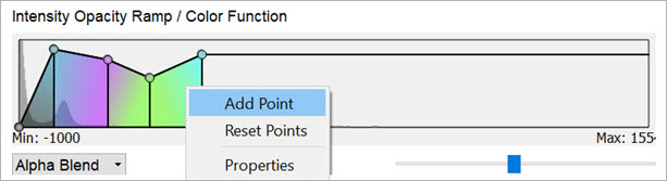
Add Point When adding a new point to the function, a color picker window opens which by default assigns interpolated color between the two surrounding points. Users are allowed to change this color. Also, the color of any of the function points can be changed by right-clicking it and selecting Color. To remove a point from the histogram, right-click on the point to be deleted and select Delete Point.
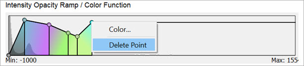
Delete Point -
Blending: Controls how volume blend together. Options are: Max or Alpha.
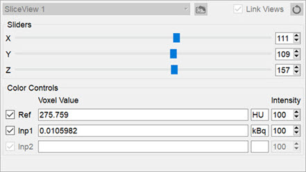
Color Controls
The Color Controls section provides users with the ability to define tissues and their corresponding coloring properties (opacity and RGB), for volume rendering.
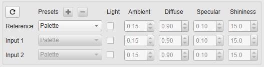
VivoQuant volume renderer allows for manipulating 3 data sets at the same time: Reference, Input 1 and Input 2. Users can select canned tissue presets, as well as creating and saving custom tissue properties, and editing existing tissue opacity and color functions.
Tissue properties can be selected from the Presets combo box.
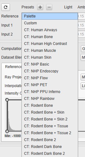
Users can select any of the following preset options:
-
Palette: Syncs with the palette selected in the Data Manager and reacts to min/max changes. This option does not allow custom coloring for the function. New presets cannot be added based on this option. Therefore the Add Preset and Remove Preset buttons are disabled.
-
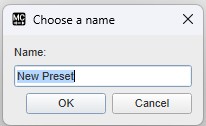
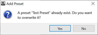
Custom: Allows for coloring from the current function. The default colors will be those of the palette option if no presets were selected beforehand. This is the only option that allows for adding new presets. To add a new custom preset, click on the Add Preset button. A popup window opens prompting the user to enter a name for the new custom preset.
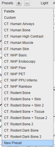
The newly created preset will then appear on the list of presets in the Presets combo box.
To remove a custom preset, click on the Remove Preset button. A popup window opens asking the user to confirm deletion of the custom preset.
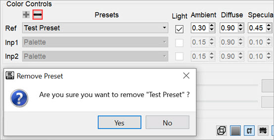
- CT Tissue Types and Species: These are presets that present CT property configurations that are specific to different tissue types and species. Some examples include: CT: Human Bone; CT: Human Muscle; CT: NHP Basics; CT: NHP PET; CT: Rodent Bone + Skin; CT: Rodent Dark Bone; among others.
Users can edit the shading settings by enabling the Light checkbox under Color Controls. The available shading and lighting settings are as follows:
| Ambient | Ambient light is the light that is scattered by the environment. It is a simple approximation of global illumination that is independent from the light position, object orientation, observer’s position or orientation. That is, ambient light has no direction. |
| Diffuse | Diffuse light is the illumination that a surface receives from a light source and reflects equally in all directions. |
| Specular | Specular light is a light that retains its reflective qualities. When this light hits a surface, reflection bounces back into the camera. Specular light is a bright spot on an object. It is the result of total reflection of incident light in a concentrate region. |
| Shininess | Shininess is a material property that determines the size and sharpness of specular highlights. |
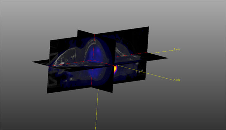
MPR View
The Multi-Planar Reconstruction View (MPR) simultaneously displays a sagittal, coronal, and transversal slice of the reconstruction. The View Control is used to change the active planes while the sliders and checkboxes across the top of the window may be used to rotate the view, display the bounding box, reset the view, and turn on/off individual planes.
The image in MPR View may be rotated by using a left-click and dragging the mouse. Similarly, panning may be controlled by holding the Shift key, using a left-click, and dragging the mouse. The zoom may be changed by using the mouse’s scroll wheel.
To change the active planes in the MPR View, use the (X,Y,Z) sliders in the View Control.